Inverted Pendulum, which is also a Lamp

Leon Kie included in arduino feedback control theory

2020-08-31 1738 words 9 minutes

Contents

Introduction

The inverted pendulum is one of the most popular demonstrations in system control, has been studied since the 1960¹ and is a prime example at unis and other research institutes. However, the inverted pendulum, which is nothing more than a pendulum that has the centre of mass above the pivot point, yet has no particular use case. To change this once in for all, I build an inverted pendulum lamp, which can be used as a normal stylish desk lamp. (The main incentive, however, wasn’t so heroic. Honestly! It sounded just like a nice project idea!)

Note

This blog post will give you a step by step recreation guide and highlights the design choices I made as well as introduce you to the implementation of the LQR Control Algorithm I used to balance the Lamp. I will also mention the resources that I used to speed up the programming part at the end of the post!

Building

Components

List of used parts

Mechanical Setup

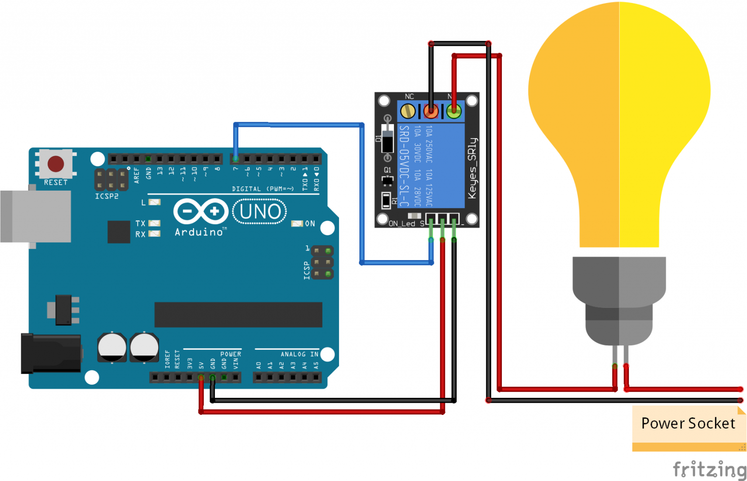
To accomplish this symbiosis between this still highly complex balancing problem and the potential usage as a design element, I first had to design a balancing cart 🚗 with a pivoting E27 socket for the lamp 💡. This brings the extra challenge of feeding a, in this case, 230V, cable through various mountings and controlling it using an ordinary relay.

Design-choices

⚙️ DV-Motor (first axel)

the L298N Motor Driver Module works up to 12V, without removing the jumper wire, therefore a 12V DV-Motor is a good choice for the setup
should have sufficient torque and RPM. In my case around 300-440 RPM (depending on your wheel size) with a 15:1 gear ratio and 10Ncm was enough
❗ be careful with the maximum current! The allowed Amps for the L298N Motor Driver Module is 2A (more information here)

📏 Contious Angle Sensor (second axel)

used to monitor the position of the cart 🚗 relative to its starting position
works like a normal potentiometer but allows for more than 360° turning angle.
not the most reliable solution as it produced high noise in the zero orientation
=> Quick-fix: use a capacitor as a low-pass filter between the ground and output voltage.

📟 Arduino

the L298 has a 5V regulator and can be used as the power supply for the Arduino (see connection diagram)
❗ don’t mount any high current consumer like the lamp 💡 or the motor ⚙ to the 5V output of the board it is not made for such high currents.

📏 Potentiometer 50k (linear)

used to detect the angle of the pendulum
additionally used as a mount for the pendulum

🔌 Capsule Slip Ring AC 240V

the lamp 💡 is powered by an isolated electric circuit with 240V AC
the slip ring feeds the power thought the rotational pivot point
also used as a mount for the pendulum

🔌 Relay

isolates the 12V DC and the 240V AC
is triggerd by the Arduino

Connecting Motor Driver Board

Connecting Potentiometer

Integration of Relay²

Control Algorithm

In the following section, I will give a brief introduction to the theory of the LQR Controller and provide you with my recommended resources which help you determine the coefficients of the feedback regulator!

Mathematical representation

The simplified system consists of an inverted pendulum which is connected to a motorized card. Without further inspection, we can recognize that we are looking at an unstable system. If the cart is not moved it is nearly impossible to balance the pendulum in the upright position. The objective is it now to design a feedback controller which accelerates the cart enough so that the angle $ \phi $ of the pendulum is close to 180°.

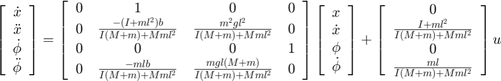
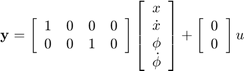
For this we first have to define the nonlinear model:

List of Variables

M mass of the cart
m mass of the pendulum
b coefficient of friction for cart
l length to pendulum centre of mass
I mass moment of inertia of the pendulum
F force applied to the cart
x cart position coordinate
$\theta$ pendulum angle from vertical (down)
u (input) here equivalent to the Force F

LQR Controller

The LQR or Linear quadratic regulator is one of many optimal control techniques, which takes into account the whole state vector and computes the control decision based on a linear model. For non-linear plants like our inverted pendulum, the system equations first have to be linearized about the upright (unstable) equilibrium. This consequently means that our LQR controller is only sufficient within small deviations around the upright position. After linearizing we have to calculate the gains $K$, this is done using the script linked here. With all that done, we now can compute the input voltage of the Motor using the following equation:

$$ u = -Kx $$

A deeper dive into the theory behind the calculation of the linearized model can be found here!

Determine grains

The script which already includes the linearized model to determine the gains for the LQR Controller can be found here!

Tip

When you calculate the model-specific gains $K$ it is very important that you measure the weight ⚖ of the cart 🚗 and the pendulum + lamp 💡 very precisely as the controller is very sensitive!

To furthermore approve your parameters the script [controlled-cart-pendulum.py] from a similar project³ simulates the control behaviour.

DC-Motor system identification

The LQR Controller takes as an input the Force F of the DC-Motor. Therefore the next step is to find the underlying DC-Motor model and estimate the corresponding system parameters. Then the Arduino can change the speed of the engine using the PWM signal.

We can model a standard DC-Motor using the following equation: $$ \frac{d w}{d t}\left(J+m r^{2}\right)+w\left(B+\frac{k^{2}}{R}\right)=\frac{k U}{R} $$

Simplifying this further:

To determine the parameters a,b,c we can record several velocity curves with different input voltages. Using the following plot and theses scripts [dc_motor_lqr_control.py,estimate_params.py] we can now find the exact model parameters!

Credits to zjor for creating the scripts³

Code

The code is based on an existing Arduino project³

  1
  2
  3
  4
  5
  6
  7
  8
  9
 10
 11
 12
 13
 14
 15
 16
 17
 18
 19
 20
 21
 22
 23
 24
 25
 26
 27
 28
 29
 30
 31
 32
 33
 34
 35
 36
 37
 38
 39
 40
 41
 42
 43
 44
 45
 46
 47
 48
 49
 50
 51
 52
 53
 54
 55
 56
 57
 58
 59
 60
 61
 62
 63
 64
 65
 66
 67
 68
 69
 70
 71
 72
 73
 74
 75
 76
 77
 78
 79
 80
 81
 82
 83
 84
 85
 86
 87
 88
 89
 90
 91
 92
 93
 94
 95
 96
 97
 98
 99
100
101
102
103
104
105
106
107
108
109
110
111
112
113
114
115
116
117
118
119
120
121
122
123
124
125
126
127
128
129
130
131
132
133
134
135
136
137
138
139
140
141
142
143
144
145
146
147
148
149
150
151
152
153
154
155
156
157
158
159
160
161
162
163
164
165
166
167
168
169
170
171
172
173
174
175
176
177
178
179
180
181
182
183
184
185
186
187
188
189
190
191
192
193
194
195
196
197
198
199
200
201
202
203
204
205
206
207
208


#define A 9   
#define B 1.0 
#define C 2.1 

#define Kth 61.20847945 
#define Kw  10.42165907
#define Kx  16.2303454
#define Kv  13.43669139 

#define Ki  0
#define PI 3.1415926535897932384626433832795


//define pins
int speed = 9;
int front = 6;
int back  = 7;
int lamp = 2;


//define constans
float wheelCirc = 141.37;
float THETA_THRESHOLD = PI / 8;

unsigned long now = 0L;
unsigned long lastTimeMicros = 0L;


//init States
float x=0;
float d_x;
float phi;
float d_phi;
float phi_sum=0;

//usefull variables
float pos_last1;
float pos_last2;
float pos_last3;
float pos_last4;
float last_phi;

float control, u, dt , v_soll;


// the setup routine runs once when you press reset:
void setup() {
  // initialize serial communication at 9600 bits per second:
  Serial.begin(9600);
  pinMode(speed, OUTPUT);
  pinMode(front, OUTPUT);
  pinMode(back, OUTPUT);
  pinMode(lamp, OUTPUT);
  digitalWrite(lamp,HIGH);
  digitalWrite(front, LOW);
  digitalWrite(back, LOW);
  
  pos_last1= mapf(analogRead(A1),0,1023,0,wheelCirc)/1000;
  pos_last2=pos_last1;
  pos_last3=pos_last1;
  pos_last4=pos_last1;
  last_phi= mapf(analogRead(A0)-512+4 , -512, 512, -PI ,PI );
  lastTimeMicros = 0L;
  
  //Debugging

  //Serial.print("x");Serial.print("\t");
  //Serial.print("dx");Serial.println("\t");
  //Serial.print("Kv*d_x");Serial.print("\t");
  //Serial.print("Kth*phi");Serial.print("\t");
  //Serial.print("Kw*d_phi");Serial.print("\t");
  //Serial.print("control");Serial.print("\t");
  //Serial.print("u");Serial.println("\t");
}


float mapf(float x, float in_min, float in_max, float out_min, float out_max) {
  return (x - in_min) * (out_max - out_min) / (in_max - in_min) + out_min;
}


void driveMotor(float pwm_out){
  analogWrite(speed, fabs(pwm_out));
    if (pwm_out > 0) {
      digitalWrite(front, HIGH);
      digitalWrite(back, LOW);
    }else if (pwm_out < 0) {
      digitalWrite(front, LOW);
      digitalWrite(back, HIGH);
    }else{
      digitalWrite(front, LOW);
      digitalWrite(back, LOW);
      
    }
  
}


boolean isControllable(float phi) {
  return fabs(phi) < THETA_THRESHOLD;
}

float saturate(float v, float maxValue) {
  if (fabs(v) > maxValue) {
    return (v > 0) ? maxValue : -maxValue;
  } else {
    return v;
  }
}


float derivative(float x_new, float x_old, float dt){
  
  float d_temp= x_new - x_old;
  float d_pos = 0;
  
  if (fabs(d_temp) < fabs(d_temp+wheelCirc/1000) and (fabs(d_temp) < fabs(d_temp-wheelCirc/1000))){
    d_pos= d_temp;
  }else if (fabs(d_temp+wheelCirc/1000) < fabs(d_temp-wheelCirc/1000)){
    d_pos= (d_temp+wheelCirc/1000);
  }else {
    d_pos= (d_temp-wheelCirc/1000);
  }
  
  if (fabs(d_pos/dt)>1.1){
    d_pos= -d_x*dt;
  } 
  
  return - d_pos/dt;
}

void updateStates(float dt){
  

  //read sensor input (Angle of wheel)
  float sensor_x = analogRead(A1);
  float pos_new =mapf(sensor_x,0,1023,0,wheelCirc)/1000;

  //smoothing the signal input 
  float pos_avg= (pos_last1+pos_last2+pos_last3+pos_last4)/4; 
  float d_x_2 = derivative(pos_new, pos_last2,2*dt);
  float d_x_3 = derivative(pos_new, pos_last3,3*dt);
  d_x = (d_x_2+d_x_3)/2;
  
  //update state variables
  x = x + dt*d_x;
  pos_last4=pos_last3;
  pos_last3=pos_last2;
  pos_last2=pos_last1;
  pos_last1=pos_new;
  
  //read sensor phi
  float sensor_phi = analogRead(A0) - 512;
  phi = mapf(sensor_phi+8 , -512, 512, -PI, PI ); // map sensor input to correct mean an variance 
  

  d_phi=(phi-last_phi)/dt;
  last_phi= phi;
  
  phi_sum=phi_sum+dt*phi;
  if (isControllable(phi)){
    phi_sum=0;
  }
  
  //Debugging

  //Serial.print(sensor_x, 4);Serial.print("\t");
  //Serial.print(sensor_x, 4);Serial.print("\t");
  //Serial.print(pos_new, 4);Serial.print("\t");
  //Serial.print(d_x*1000, 4);Serial.println("\t");
  //Serial.print(d_x_2*1000, 4);Serial.print("\t");
  //Serial.print(d_x_3*1000, 4);Serial.println("\t");
  //Serial.print(d_x_4*1000, 4);Serial.println("\t");
  //Serial.print(phi, 4);Serial.print("\t");
  //Serial.print(d_phi, 4);Serial.print("\t");

}

// the loop routine runs over and over again forever:
void loop() {
  now = micros();
  dt = (1.0*(now - lastTimeMicros))/ 1000000;
  updateStates(dt);
  
  
  
  
  if (isControllable(phi)) {
    digitalWrite(lamp, LOW);
    
    control = (Kx * x + Kv * d_x + Kth * phi + Kw * d_phi);
    u = (control + A * d_x + copysignf(C, d_x)) / B;
    u = 255.0 * u / 12;
    
    v_soll = saturate(u, 254);
    driveMotor(v_soll);
  } else {
    v_soll= 0;
    driveMotor(v_soll);
    digitalWrite(lamp, HIGH);
  }
  



  lastTimeMicros = now;
  delay(5);        // delay in between reads for stability
}